Linear Programming

Introduction to LP Problems

Standard Form vs General Form

KEY: equivalence of (S) and (G)

Any linear programming problem, i.e

can be expressed compactly in both standard form and general form.

Definition 1.1.1 (General Form) A linear programming problem can be written as

$$\begin{array}{rll} \operatorname{minimize} & \mathbf{c}^{\prime} \mathbf{x} \\ \text { subject to } & \mathbf{A x} \geq \mathbf{b} \end{array}$$

Definition 1.1.2 (Standard Form) A linear programming problem of the form

$$\begin{array}{rr} \operatorname{minimize} & \mathbf{c}^{\prime} \mathbf{x} \\ \text { subject to } & \mathbf{A x}=\mathbf{b} \\ & \mathbf{x} \geq \mathbf{0} \end{array}$$

is said to be in standard form.

Polyhedron and convex sets

KEY: definition of polyhedron; definition of convex set.

We might as well revisit some definitions in convex optimization.

Definition 1.2 (Convexity and Concavity)

(a) A function $f: \Re^{n} \mapsto \Re$ is called convex if for every $\mathbf{x}, \mathbf{y} \in \Re^{n}$, and every $\lambda \in[0,1]$, we have

$$f(\lambda \mathbf{x}+(1-\lambda) \mathbf{y}) \leq \lambda f(\mathbf{x})+(1-\lambda) f(\mathbf{y})$$

(b) A function $f: \Re^{n} \mapsto \Re$ is called concave if for every $\mathbf{x}, \mathbf{y} \in \Re^{n}$, and every $\lambda \in[0,1]$, we have

$$f(\lambda \mathbf{x}+(1-\lambda) \mathbf{y}) \geq \lambda f(\mathbf{x})+(1-\lambda) f(\mathbf{y})$$

We also start with the formal definition of a polyhedron as well as a convex set.

Definition 1.3 (Polyhedron) A polyhedron is a set that can be described in the form $\left\{\mathbf{x} \in \Re^{n} \mid \mathbf{A} \mathbf{x} \geq \mathbf{b}\right\}$, where $\mathbf{A}$ is an $m \times n$ matrix and $\mathbf{b}$ is a vector in $\Re^{m}$.

Definition 1.4 (Convex Set) A set $S \subset \Re^{n}$ is convex if for any $\mathbf{x}, \mathbf{y} \in S$, and any $\lambda \in[0,1]$, we have $\lambda \mathbf{x}+(1-\lambda) \mathbf{y} \in S$.

A polyhedron can either “extend to infinity,” or can be confined in a finite region. The definition that follows refers to this distinction.

Definition 1.5 (Boundedness) A set $S \subset \Re^{n}$ is bounded if there exists a constant $K$ such that the absolute value of every component of every element of $S$ is less than or equal to $K$.

The convex set also provide some interesting facts.

Theorem 1.1

(a) The intersection of convex sets is convex.

(b) Every polyhedron is a convex set.

(c) A convex combination of a finite number of elements of a convex set also belongs to that set.

Extreme Points and Basic Feasible Solutions

KEY: BFS = extreme point; geometric property of extreme point.

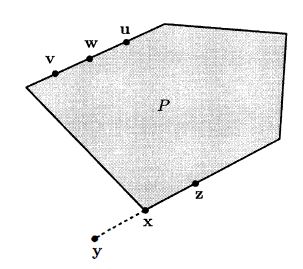
Our first definition defines an extreme point of a polyhedron as a point that cannot be expressed as a convex combination of two other elements of the polyhedron. This definition is entirely geometric and does not refer to a specific representation of a polyhedron in terms of linear constraints.

Definition 1.6 (Extreme Point) Let $P$ be a polyhedron. A vector $\mathrm{x} \in P$ is an extreme point of $P$ if we cannot find two vectors $y, z \in P$, both different from $\mathbf{x}$, and a scalar $\lambda \in[0,1]$, such that $\mathbf{x}=\lambda \mathbf{y}+(1-\lambda) \mathbf{z}$.

To introduce the definition of basic feasible solution, we will first introduce the notation of active set.

Definition 1.7 (Active Set) If a vector $\mathbf{x}^{*}$ satisfies $\mathbf{a}_{i}^{\prime} \mathbf{x}^{*}=b_{i}$ for some $i$ in $M_{1}, M_{2}$, or $M_{3}$, we say that the corresponding constraint is active at $\mathbf{x}^{*}$. $I=\left\{i \mid \mathbf{a}_{i}^{\prime} \mathbf{x}^{*}=b_{i}\right\}$ is the set of indices of constraints that are active at $x^*$, or active set.

From basic linear algebra knowledge, we can have the following theorem.

Theorem 1.2 Let $\mathbf{x}^{*}$ be an element of $\Re^{n}$ and let $I=\left\{i \mid \mathbf{a}_{i}^{\prime} \mathbf{x}^{*}=b_{i}\right\}$ be the active set of $\mathbf{x}^{*}$. Then, the following are equivalent:

(a) There exist $n$ vectors in the set $\left\{\mathbf{a}_{i} \mid i \in I\right\}$, which are linearly independent.

(b) The span of the vectors $\mathbf{a}_{i}, i \in I$, is all of $\Re^{n}$, that is, every element of $\Re^{n}$ can be expressed as a linear combination of the vectors $\mathbf{a}_{i}, i \in I$.

(c) The system of equations $\mathbf{a}_{i}^{\prime} \mathbf{x}=b_{i}, i \in I$, has a unique solution.

We are now ready to provide an algebraic definition of a corner point, as a feasible solution at which there are $n$ linearly independent active constraints. However, note that this procedure has no guarantee of leading to a feasible vector. Basic solution is a totally different notion with basic feasible solution.

Definition 1.8 (Basic Solution vs Basic Feasible Solution) Consider a polyhedron $P$ defined by linear equality and inequality constraints, and let $\mathbf{x}^{*}$ be an element of $\Re^{n}$.

(a) The vector $\mathrm{x}^{*}$ is a basic solution if:

​ (i) All equality constraints are active;

​ (ii) Out of the constraints that are active at $\mathbf{x}^{*}$, there are $n$ of them that are linearly independent.

(b) If $\mathbf{x}^{*}$ is a basic solution that satisfies all of the constraints, we say that it is a basic feasible solution.

These two different definitions are, however, meant to capture the same concept geometrically and algebraically. This could be verified by contradiction.

Theorem 1.3 Let $P$ be a nonempty polyhedron and let $\mathbf{x}^{*} \in P$. Then, the following are equivalent:

(a) $\mathbf{x}^{*}$ is an extreme point;

(b) $\mathbf{x}^{*}$ is a basic feasible solution.

And we can easily derive the corollary.

Corollary 1.1 Given a finite number of linear inequality constraints, there can only be a finite number of basic or basic feasible solutions.

Standard Form Polyhedron

KEY: Theorem 1.4.

Recall that at any basic solution, there must be $n$ linearly independent constraints that are active. Furthermore, every basic solution must satisfy the equality constraints $\mathbf{A} \mathbf{x}=\mathbf{b}$, which provides us with $m$ linear independent active constraints. Therefore, there are $n-m$ more constraints from $n$ constraints of $x_i\ge 0$.

Theorem 1.4 Consider the constraints $\mathbf{A x}=\mathbf{b}$ and $\mathbf{x} \geq \mathbf{0}$ and assume that the $m \times n$ matrix $\mathbf{A}$ has linearly independent rows. A vector $\mathbf{x} \in \Re^{n}$ is a basic solution if and only if we have $\mathbf{A} \mathbf{x}=\mathbf{b}$, and there exist indices $B(1), \ldots, B(m)$ such that:

(a) The columns $\mathbf{A}_{B(1)}, \ldots, \mathbf{A}_{B(m)}$ are linearly independent;

(b) If $i \neq B(1), \ldots, B(m)$, then $x_{i}=0$.

In this way, we can construct basic feasible solutions in the following way.

1. Choose $m$ linearly independent columns $\mathbf{A}_{B(1)}, \ldots, \mathbf{A}_{B(m)}$.
2. Let $x_{i}=0$ for all $i \neq B(1), \ldots, B(m)$.
3. Solve the system of $m$ equations $\mathbf{A} \mathbf{x}=\mathbf{b}$ for the unknowns $x_{B(1)}$, $\ldots, x_{B(m)}$.

We can also obtain an $m \times m$ matrix $\mathbf{B}$, called a basis matrix, by arranging the $m$ basic columns next to each other. We can similarly define a vector $\mathbf{x}_{B}$ with the values of the basic variables. Thus,

The basic variables are determined by solving the equation $\mathbf{B} \mathbf{x}_{B}=\mathbf{b}$ whose unique solution is given by

Existence of Extreme Points

KEY: has extreme point $\leftrightarrow$ does not contain a line; a line has at most two intersection with a polyhedron.

We need the following definition

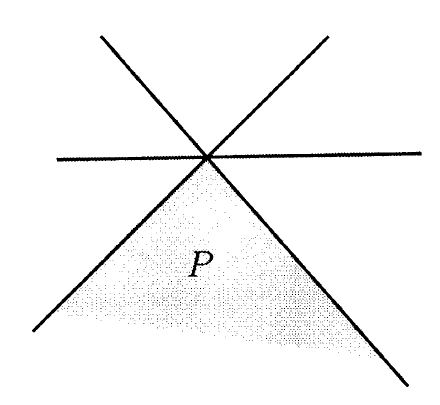
Definition 1.9 A polyhedron $P \subset \Re^{n}$ contains a line if there exists a vector $\mathbf{x} \in P$ and a nonzero vector $\mathbf{d} \in \Re^{n}$ such that $\mathbf{x}+\lambda \mathbf{d} \in P$ for all scalars $\lambda$.

to formulate the following theorem.

Theorem 1.5 Suppose that the polyhedron $P=\left\{\mathbf{x} \in \Re^{n} \mid \mathbf{a}_{i}^{\prime} \mathbf{x} \geq\right.$ $\left.b_{i}, i=1, \ldots, m\right\}$ is nonempty. Then, the following are equivalent:

(a) The polyhedron $P$ has at least one extreme point.

(b) The polyhedron $P$ does not contain a line.

(c) There exist $n$ vectors out of the family $\mathbf{a}_{1}, \ldots, \mathbf{a}_{m}$, which are linearly independent.

Since a bounded polyhedron does not contain a line, we will have the following corollary

Corollary 1.2 Every nonempty bounded polyhedron and every nonempty polyhedron in standard form has at least one basic feasible solution.

Optimality of Extreme Points

If $P=\left\{\mathbf{x} \in \Re^{n} \mid \mathbf{A} \mathbf{x} \geq \mathbf{b}\right\}$ is the feasible set and $v$ is the optimal value of the cost $\mathbf{c}^{\prime} \mathbf{x}$. Then, $Q=\left\{\mathbf{x} \in \Re^{n} \mid \mathbf{A} \mathbf{x} \geq \mathbf{b}, \mathbf{c}^{\prime} \mathbf{x}=v\right\}$ is also a polyhedron. With this, we can prove the following theorem that, as long as a linear programming problem has an optimal solution and as long as the feasible set has at least one extreme point, we can always find an optimal solution within the set of extreme points of the feasible set .

Theorem 1.6 Consider the linear programming problem of minimizing $\mathbf{c}^{\prime} \mathbf{x}$ over a polyhedron $P$. Suppose that $P$ has at least one extreme point and that there exists an optimal solution. Then, there exists an optimal solution which is an extreme point of $P$.

A stronger result shows that the existence of an optimal solution can be taken for granted, as long as the optimal cost is finite.

Theorem 1.7 Consider the linear programming problem of minimizing $\mathbf{c}^{\prime} \mathbf{x}$ over a polyhedron $P$. Suppose that $P$ has at least one extreme point. Then, either the optimal cost is equal to $-\infty$, or there exists an extreme point which is optimal.

As any linear programming problem can be transformed into an equivalent problem in standard form, we will have the following corollary.

Corollary 1.3 Consider the linear programming problem of minimizing $\mathbf{c}^{\prime} \mathbf{x}$ over a nonempty polyhedron. Then, either the optimal cost is equal to $-\infty$ or there exists an optimal solution.

Miscellaneous

One might be doubtful why $\mathbf{A}$ is always assumed to be full row rank. The following theorem shows that the full row rank assumption on the matrix $\mathbf{A}$ results in no loss of generality.

Theorem 1.8 Let $P=\{\mathbf{x} \mid \mathbf{A} \mathbf{x}=\mathbf{b}, \mathbf{x} \geq \mathbf{0}\}$ be a nonempty polyhedron, where $\mathbf{A}$ is a matrix of dimensions $m \times n$, with rows $\mathbf{a}_{1}^{\prime}, \ldots, \mathbf{a}_{m}^{\prime}$. Suppose that $\operatorname{rank}(\mathbf{A})=k<m$ and that the rows $\mathbf{a}_{i_{1}}^{\prime}, \ldots, \mathbf{a}_{i_{k}}^{\prime}$ are linearly independent. Consider the polyhedron

$$Q=\left\{\mathbf{x} \mid \mathbf{a}_{i_{1}}^{\prime} \mathbf{x}=b_{i_{1}}, \ldots, \mathbf{a}_{i_{k}}^{\prime} \mathbf{x}=b_{i_{k}}, \mathbf{x} \geq \mathbf{0}\right\}$$

Then $Q=P$.

In some cases, the basic feasible solution is degenerate.

Definition 1.10 (Degeneracy) Consider the standard form polyhedron $P=\{\mathbf{x} \in$ $\left.\Re^{n} \mid \mathbf{A x}=\mathbf{b}, \mathbf{x} \geq \mathbf{0}\right\}$ and let $\mathbf{x}$ be a basic solution. Let $m$ be the number of rows of $\mathbf{A}$. The vector $\mathbf{x}$ is a degenerate basic solution if more than $n-m$ of the components of $\mathbf{x}$ are zero.

An important comment is that degeneracy is not a pure geometric property. That is to say, a degenerate basic feasible solution under one representation could be nondegenerate under another representation.

Simplex Method

Optimality conditions

**KEY: feasible direction; **

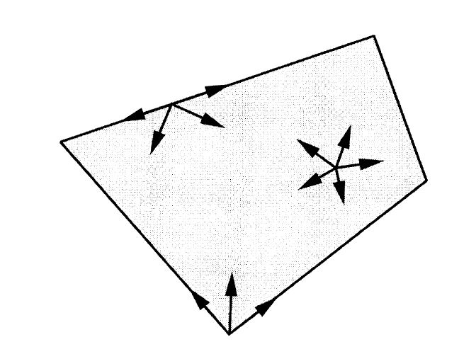
Suppose that we are at a point $\mathbf{x} \in P$ and that we contemplate moving away from $\mathbf{x}$, in the direction of a vector $\mathbf{d} \in \Re^{n}$. Clearly, we should only consider those choices of $\mathbf{d}$ that do not immediately take us outside the feasible set.

Definition 2.1 (Feasible Direction) Let $\mathrm{x}$ be an element of a polyhedron $P$. A vector $\mathbf{d} \in \Re^{n}$ is said to be a feasible direction at $\mathrm{x}$, if there exists a positive scalar $\theta$ for which $\mathbf{x}+\theta \mathbf{d} \in P$.

Given that we are only interested in feasible solutions, we require $\mathbf{A}(\mathbf{x}+\theta \mathbf{d})=\mathbf{b}$, and since $\mathbf{x}$ is feasible, we also have $\mathbf{A} \mathbf{x}=\mathbf{b}$. Thus, for the equality constraints to be satisfied for $\theta>0$, we need $\mathbf{A d}=\mathbf{0}$. If we want to move to adjacent extreme point, it must satisfy the condition that $d_{j}=1$, and $d_{i}=0$ for all other non-basic indices $i$. Then,

Since the basis matrix $\mathbf{B}$ is invertible, we obtain

Definition 2.2 (Reduced Cost) Let $\mathbf{x}$ be a basic solution, let $\mathbf{B}$ be an associated basis matrix, and let $\mathbf{c}_{B}$ be the vector of costs of the basic variables. For each $j$, we define the reduced cost $\bar{c}_{j}$ of the variable $x_{j}$ according to the formula

$$\bar{c}_{j}=c_{j}-\mathbf{c}_{B}^{\prime} \mathbf{B}^{-1} \mathbf{A}_{j}$$

With reduced cost, we can provide optimality conditions of linear programming.

Theorem 2.1 Consider a basic feasible solution $\mathrm{x}$ associated with a basis matrix $\mathbf{B}$, and let $\overline{\mathbf{c}}$ be the corresponding vector of reduced costs.

(a) If $\overline{\mathbf{c}} \geq \mathbf{0}$, then $\mathbf{x}$ is optimal.

(b) If $\mathbf{x}$ is optimal and nondegenerate, then $\overline{\mathbf{c}} \geq \mathbf{0}$.

Proof.

(a) We assume that $\overline{\mathbf{c}} \geq \mathbf{0}$, we let $\mathbf{y}$ be an arbitrary feasible solution, and we define $\mathbf{d}=\mathbf{y}-\mathbf{x}$. Feasibility implies that $\mathbf{A x}=\mathbf{A y}=\mathbf{b}$ and, therefore, $\mathbf{A d}=\mathbf{0}$. The latter equality can be rewritten in the form

$$\mathbf{B d}_{B}+\sum_{i \in N} \mathbf{A}_{i} d_{i}=\mathbf{0}$$

where $N$ is the set of indices corresponding to the nonbasic variables under the given basis. Since B is invertible, we obtain

$$\mathbf{d}_{B}=-\sum_{i \in N} \mathbf{B}^{-1} \mathbf{A}_{i} d_{i}$$

and

$$\mathbf{c}^{\prime} \mathbf{d}=\mathbf{c}_{B}^{\prime} \mathbf{d}_{B}+\sum_{i \in N} c_{i} d_{i}=\sum_{i \in N}\left(c_{i}-\mathbf{c}_{B}^{\prime} \mathbf{B}^{-1} \mathbf{A}_{i}\right) d_{i}=\sum_{i \in N} \bar{c}_{i} d_{i}$$

For any nonbasic index $i \in N$, we must have $x_{i}=0$ and, since $\mathbf{y}$ is feasible, $y_{i} \geq 0$. Thus, $d_{i} \geq 0$ and $\bar{c}_{i} d_{i} \geq 0$, for all $i \in N$. We conclude that $\mathbf{c}^{\prime}(\mathbf{y}-\mathbf{x})=\mathbf{c}^{\prime} \mathbf{d} \geq 0$, and since $\mathbf{y}$ was an arbitrary feasible solution, $\mathbf{x}$ is optimal.

(b) Suppose that $\mathrm{x}$ is a nondegenerate basic feasible solution and that $\bar{c}_{j}<0$ for some $j$. Since the reduced cost of a basic variable is always zero, $x_{j}$ must be a non-basic variable and $\bar{c}_{j}$ is the rate of cost change along the $j$ th basic direction. Since $\mathrm{x}$ is nondegenerate, the $j$ th basic direction is a feasible direction of cost decrease, as discussed earlier. By moving in that direction, we obtain feasible solutions whose cost is less than that of $\mathbf{x}$, and $\mathbf{x}$ is not optimal.

Simplex Method (Naive)

An iteration of the simplex method

1. In a typical iteration, we start with a basis consisting of the basic columns $\mathbf{A}_{B(1)}, \ldots, \mathbf{A}_{B(m)}$, and an associated basic feasible solution $\mathrm{x}$.
2. Compute the reduced costs $\bar{c}_{j}=c_{j}-\mathbf{c}_{B}^{\prime} \mathbf{B}^{-1} \mathbf{A}_{j}$ for all non-basic indices $j$. If they are all nonnegative, the current basic feasible solution is optimal, and the algorithm terminates; else, choose some $j$ for which $\bar{c}_{j}<0$.
3. Compute $\mathbf{u}=-\mathbf{d_B}=\mathbf{B}^{-1} \mathbf{A}_{j}$. If no component of $\mathbf{u}$ is positive, we have $\theta^{*}=\infty$, the optimal cost is $-\infty$, and the algorithm terminates.
4. If some component of $\mathbf{u}$ is positive, let

$$\theta^{*}=\min _{\left\{i=1, \ldots, m \mid u_{i}>0\right\}} \frac{x_{B(i)}}{u_{i}} .$$

5. Let $\ell$ be such that $\theta^{*}=x_{B(\ell)} / u_{\ell}$. Form a new basis by replacing $\mathbf{A}_{B(\ell)}$ with $\mathbf{A}_{j}$. If $\mathbf{y}$ is the new basic feasible solution, the values of the new basic variables are $y_{j}=\theta^{*}$ and $y_{B(i)}=x_{B(i)}-\theta^{*} u_{i}$, $i \neq \ell$.

If we define $\bar{B}(i)= \begin{cases}B(i), & i \neq \ell \\ j, & i=\ell,\end{cases}$ which is the new basis of the new basic feasible solution. This can be verified by the following theorem.

Theorem 2.2

(a) The columns $\mathbf{A}_{B(i)}, i \neq \ell$, and $\mathbf{A}_{j}$ are linearly independent and, therefore, $\overline{\mathbf{B}}$ is a basis matrix.

(b) The vector $\mathbf{y}=\mathbf{x}+\theta^{*} \mathbf{d}$ is a basic feasible solution associated with the basis matrix $\overline{\mathbf{B}}$.

The problem of this naive implementation is that the matrix inverse has $O(n^3)$ complexity, thus resulting in $O(m^3 + mn)$ computational effort per iteration. Nevertheless, simplex method is guaranteed convergence.

Theorem 2.3 (Convergence of Simplex Method) Assume that the feasible set is nonempty and that every basic feasible solution is nondegenerate. Then, the simplex method terminates after a finite number of iterations. At termination, there are the following two possibilities:

(a) We have an optimal basis $\mathbf{B}$ and an associated basic feasible solution which is optimal.

(b) We have found a vector $\mathbf{d}$ satisfying $\mathbf{A d}=\mathbf{0}, \mathbf{d} \geq \mathbf{0}$, and $\mathbf{c}^{\prime} \mathbf{d}<0$, and the optimal cost is $-\infty$.

Simplex Method (Revised)

Notice that since $\mathbf{B}^{-1} \mathbf{B}=\mathbf{I}$, we have the property that $\mathbf{B}^{-1} \mathbf{A}_{B(i)}$ is the $i$ th unit vector $\mathbf{e}_{i}$. Using this observation, we have

where $\mathbf{u}=-\mathbf{d_B}=\mathbf{B}^{-1} \mathbf{A}_{j}$. Since the result is the identity, we have $\mathbf{Q B}{ }^{-1} \overline{\mathbf{B}}=\mathbf{I}$, which yields $\mathbf{Q} \mathbf{B}^{-1}=\overline{\mathbf{B}}^{-1}$. We can update $\mathbf{B}^{-1}$ to $\overline{\mathbf{B}}^{-1}$ by row operations with $\mathbf{Q}$.

This will reduce the operation per iteration to $O(m^2+mn)$.

Simplex Method (Tableau)

Another implementation of simplex method is called full tableau. Here, instead of maintaining and updating the matrix $\mathbf{B}^{-1}$, we maintain and update the $m \times(n+1)$ matrix

with columns $\mathbf{B}^{-1} \mathbf{b}$ and $\mathbf{B}^{-1} \mathbf{A}_{1}, \ldots, \mathbf{B}^{-1} \mathbf{A}_{n}$. This matrix is called the simplex tableau. Note that the column $\mathbf{B}^{-1} \mathbf{b}$, called the zeroth column, contains the values of the basic variables.

It is customary to augment the simplex tableau by including a top row, to be referred to as the zeroth row. The entry at the top left corner contains the value $-\mathbf{c}_{B}^{\prime} \mathbf{x}_{B}$, which is the negative of the current cost. The rest of the zeroth row is the row vector of reduced costs, that is, the vector $\overline{\mathbf{c}}^{\prime}=\mathbf{c}^{\prime}-\mathbf{c}_{B}^{\prime} \mathbf{B}^{-1} \mathbf{A}$. Thus, the structure of the tableau is:

Complexity

Finding an Initial Basic Feasible Solution (Two-Phase Algorithm)

Consider the problem

By possibly multiplying some of the equality constraints by $-1$, we can assume, without loss of generality, that $\mathbf{b} \geq \mathbf{0}$. We now introduce a vector $\mathbf{y} \in \Re^{m}$ of artificial variables and use the simplex method to solve the auxiliary problem

Initialization is easy for the auxiliary problem: by letting $\mathbf{x}=\mathbf{0}$ and $\mathbf{y}=\mathbf{b}$, we have a basic feasible solution and the corresponding basis matrix is the identity.

If $\mathbf{x}$ is a feasible solution to the original problem, this choice of $\mathbf{x}$ together with $\mathbf{y}=\mathbf{0}$, yields a zero cost solution to the auxiliary problem. Therefore, if the optimal cost in the auxiliary problem is nonzero, we conclude that the original problem is infeasible. Otherwise, the solution $\mathbf{x}$ will be a basic feasible solution.

Dual Simplex Method

The Dual Problem

Let $\mathbf{A}$ be a matrix with rows $\mathbf{a}_{i}^{\prime}$ and columns $\mathbf{A}_{j}$. Given a primal problem with the structure shown on the left, its dual is defined to be the maximization problem shown on the right:

An interesting fact from the above table is

Theorem 3.1 If we transform the dual into an equivalent minimization problem and then form its dual, we obtain a problem equivalent to the original problem.

And this theorem can be even stronger.

Theorem 3.2 Suppose that we have transformed a linear programming problem $\Pi_{1}$ to another linear programming problem $\Pi_{2}$, by a sequence of transformations of the following types:

(a) Replace a free variable with the difference of two nonnegative variables.

(b) Replace an inequality constraint by an equality constraint involving a nonnegative slack variable.

(c) If some row of the matrix $\mathbf{A}$ in a feasible standard form problem is a linear combination of the other rows, eliminate the corresponding equality constraint.

Then, the duals of $\Pi_{1}$ and $\Pi_{2}$ are equivalent, i.e., they are either both infeasible, or they have the same optimal cost.

Duality Theorem

We have discussed too much duality theorems in convex optimization course, so I will just list out several theorems for reference.

Theorem 3.3 (Weak duality) If $\mathrm{x}$ is a feasible solution to the primal problem and $\mathbf{p}$ is a feasible solution to the dual problem, then

$$\mathbf{p}^{\prime} \mathbf{b} \leq \mathbf{c}^{\prime} \mathbf{x}$$

Theorem 3.4 (Strong duality) If a linear programming problem has an optimal solution, so does its dual, and the respective optimal costs are equal.

Theorem 3.5 (Complementary slackness) Let $x$ and $\mathbf{p}$ be feasible solutions to the primal and the dual problem, respectively. The vectors $\mathbf{x}$ and $\mathbf{p}$ are optimal solutions for the two respective problems if and only if:

$$\begin{aligned} p_{i}\left(\mathbf{a}_{i}^{\prime} \mathbf{x}-b_{i}\right)=0, & & \forall i \\ \left(c_{j}-\mathbf{p}^{\prime} \mathbf{A}_{j}\right) x_{j}=0, & & \forall j \end{aligned}$$

Dual Simplex Method

An iteration of the dual simplex method

1. A typical iteration starts with the tableau associated with a basis matrix $\mathbf{B}$ and with all reduced costs nonnegative.
2. Examine the components of the vector $\mathbf{B}^{-1} \mathbf{b}$ in the zeroth column of the tableau. If they are all nonnegative, we have an optimal basic feasible solution and the algorithm terminates; else, choose some $\ell$ such that $x_{B(\ell)}<0$.
3. Consider the $\ell$ th row of the tableau, with elements $x_{B(\ell)}, v_{1}, \ldots$, $v_{n}$ (the pivot row). If $v_{i} \geq 0$ for all $i$, then the optimal dual cost is $+\infty$ and the algorithm terminates.
4. For each $i$ such that $v_{i}<0$, compute the ratio $\bar{c}_{i} /\left|v_{i}\right|$ and let $j$ be the index of a column that corresponds to the smallest ratio. The column $\mathbf{A}_{B(\ell)}$ exits the basis and the column $\mathbf{A}_{j}$ takes its place.
5. Add to each row of the tableau a multiple of the $\ell$ th row (the pivot row) so that $v_{j}$ (the pivot element) becomes 1 and all other entries of the pivot column become 0 .

Interior Point Method

Intro

There are three types of Interior Point Methods.

• Affine Scaling Algorithm
• Potential Reduction
• Path Following ✌
  • Primal -> Barrier Method
  • Primal-Dual -> KKT System

In this chapter, we will consider the linear programming problem in standard form.

Definition 4.1 Given polyhedron $P=\{x|Ax=b, x\ge 0\}$, the interior point of $P$ is defined as $\{x\in P|x>0\}$.

Primal Method

If we only consider the primal problem, we could integrates inequality constraints to the objective function using a logarithmic barrier $\phi(x) = \sum_{i=1}^n log(x_i)$.

Definition 4.2 (Barrier Method) To solve the LP problem in standard form, we introduce a variable $\mu > 0$, and the problem can be reformulated as $(P_\mu)$,

$$\begin{align*} \min &\quad c^Tx-\mu\sum^n_{i=1}log(x_i)\\ \textrm{s.t}&\quad Ax=b \end{align*}$$

$\forall \mu > 0$, $\exist$ unique $x(\mu)$ that solves $(P_\mu)$. When $\mu\downarrow0$, $\lim_{\mu\rightarrow0}x(\mu) = x^*$.

Primal-Dual Method

Intro

If we consider both the primal and dual problem, we could solve the KKT condition of the LP problem. Let us start with the KKT condition of the standard form.

Define the non-linear system,

Intuitively, we will use Newton method to solve non-linear systems. But here, we will first define a feasible set $\mathcal{F}=\{(x, y, s)|Ax=b, A^Ty+s=c, (x, s)>0\}$, and a central path $(x(\mu), y(\mu), s(\mu))\in \mathcal{F}$, which converges to $F(x, y, s)=0$. The central path is given by,

Definition 4.3 (Primal-Dual Method) Given the above central path. $\forall \mu > 0$, $\exist$ unique $(x(\mu), y(\mu), s(\mu))\in \mathcal{F}$ that solves $F(x(\mu), y(\mu), s(\mu))=0$. When $\mu\downarrow0$, $\lim_{\mu\rightarrow0}(x(\mu), y(\mu), s(\mu)) = (x^*, y^*, s^*)$.

Lemma 9.5 (of Bertsimas) If $x^*=x(\mu)$, $y^*=y(\mu)$ and $s^*=s(\mu)$ satisfy condition $F(x(\mu), y(\mu), s(\mu))=0$, then they are also optimal solution to $\min \, c^Tx-\mu\sum^n_{i=1}log(x_i) \quad \textrm{s.t}\, Ax=b$.

Proof: Let $x$ be an arbitrary vector that satisfies $x\ge0$ and $Ax=b$. The barrier function will be,

$$\begin{align*} B_\mu(x) &= c^Tx-\mu\sum^n_{i=1}log(x_i)\\ &= c^Tx+y^{*T}(b-Ax)-\mu\sum^n_{i=1}log(x_i)\\ &= (c-A^Ty^*)^Tx+y^{*T}b-\mu\sum^n_{i=1}log(x_i)\\ &= s^{*T}x+y^{*T}b-\mu\sum^n_{i=1}log(x_i)\\ \end{align*}$$

Take out $s^{*T}x-\mu\sum^n_{i=1}log(x_i)$, and set the derivative to zero, we have,

$$s_i^*-\mu x_i=0$$

Replacing $x_i = \dfrac{s_i^*}{\mu}$, we will have,

$$B_\mu(x)\ge n\mu+y^{*T}b-\mu\sum^n_{i=1}log(\dfrac{s_i^*}{\mu})$$

This means $x^*=\dfrac{s^*}{\mu}$ is the optimal solution to the barrier function, $B_\mu(x^*)\le B_\mu(x)$.

You may also derive the KKT condition for log-barrier method $(P_\mu)$, which is equivalent to the KKT condition in central path.

Recap: Newton’s Method

Recall that we can solve a non-linear system with Newton-Raphson method.

And for multivariable cases,

When using Newton-Raphson method, we must follow

• $JF(x_k)$ must be non-singular
• $\textrm{step-length}=1$
• Fast local convergence (super linear), but no global convergence guaranteed

Theorem 4.1 (Convergence of Newton Method) Newton method has super linear convergence, i.e $\|x_{k+1}-x_*\|_2\le M\|x_k-x_*\|^2_2$.

Proof We first define $g(x) = x-\dfrac{f(x)}{f'(x)}$. It is clear that $g'(x) = \dfrac{f(x)f''(x)}{[f'(x)]^2}$ and $g'(x_*)=0$. Then, we can find that,

$$\begin{align*} \|x_{k+1}-x_*\| &= \|x_k-\dfrac{f(x_k)}{f'(x_k)} - x_*\|\\ &= \|(x_k-\dfrac{f(x_k)}{f'(x_k)}) - (x_*-\dfrac{f(x_*)}{f'(x_*)})\|\\ &= \|g(x_k)-g(x_*)\|\\ &= \|g'(\xi)(x_k-x_*)\|\\ &= |g'(\xi)-g'(x_*)|\cdot\|x_k-x_*\|\\ &\le |g''(\eta)|\cdot\|x_k-x_*\|^2\\ &\le M\cdot\|x_k-x_*\|^2 \end{align*}$$

This method is local quadratically convergent to a solution.

We can derive one Newton step as follows.

where

is the solution to the following linear equations.

Practical Newton Method in IPM

Note that the Newton method doesn’t guarantee global convergence, we need to avoid a single $s_ix_i<0$. Otherwise, $(x_k, y_k, s_k)$ will fall out of the feasible set $\mathcal{F}=\{(x, y, s)|Ax=b, A^Ty+s=c, x, s>0\}$.

Therefore, we will introduce an intermediate variable $\mu$ to keep both optimality and centrality, and solve $s\circ x=\mu$ instead of $s\circ x=0$.

Primal-Dual IPM-Naive:

Initial state:

$$\left(x^{0}, y^{0}, s^{0}\right) \in F_{0} \quad \tau=\sigma \mu \quad \sigma \in(0,1) \quad \mu=\frac{1}{n} x^{\top} s$$

For $k=0,1, \cdots$

​ Use Newton’s Method with starting point $\left(x^{k}, y^{k}, s^{k}\right)$ to solve $F(x, y, s)=\left(\begin{array}{c}0 \\ 0 \\ \sigma \mu_{k} e\end{array}\right)$ and get,

$$\left(x^{k+1}, y^{k+1}, s^{k+1}\right) \in F^{0}$$

end

However, there is no necessity to compute the full Newton iteration. We can compute one Newton step and change the direction.

Primal-Dual IPM-Practical

(Only one iteration for inner Newton step.)

Initial state:

$$\left(x^{0}, y^{0}, s^{0}\right),\left(x^{0}, s^{0}\right)>0$$

For $k=0,1,2, \cdots$

​ Choose $\sigma_{k} \in[0,1]$, $\mu_{k}=\dfrac{1}{n} x^T s$

​ Find the Newton step of

$$\widetilde{F}_{k}(x, y, s)=\begin{pmatrix} A^{\top} y+s-c \\ A x-b \\ x \circ s-\sigma_k \cdot \mu_{k} \cdot e \end{pmatrix}=0$$

​ with the linear equations,

$$\begin{pmatrix} 0 & A^{\top} & I \\ A & 0 & 0 \\ S^{k} & 0 & X^{k} \end{pmatrix} \begin{pmatrix} \Delta x^{k} \\ \Delta y^{k} \\ \Delta s^{k} \end{pmatrix}=\begin{pmatrix} A^{\top} y+s-c \\ A x-b \\ x \circ s -\sigma_k \cdot \mu_{k} \cdot e \end{pmatrix}$$

​ Find step-size $\alpha_k$, subject to $(x_{k+1}, s_{k+1})>0$

$$\left(x_{k+1}, y_{k+1}, s_{k+1}\right)\leftarrow\left(x_{k}, y_{k}, s_{k}\right)+\alpha_{k}\left(\Delta x_{k}, \Delta y_{k}, \Delta s_{k}\right)$$

End

The following graph shows the path of convergence. If $\sigma=1$, $\tau=\mu$, the central path converges to $\mu$. If $\sigma=0$, $\tau=0$, the central path may not converge. We will discuss how to find $\sigma_k$ and $\alpha_k$ in the following section.

Path-Following Methods

For the sake of simplicity, we will define two types of neighborhoods.

We have different path-following routines. These routines will guarantee us the convergence.

• Long-step Path-Following $\rightarrow$ $\mathcal{N}_{-\infty}$
• Short-step Path-Following $\rightarrow$ $\mathcal{N}_{2}$

Long-Step Path-Following IPM

Initial State:

​ Given $\gamma\in(0, 1)$, $0<\sigma_{min}\le\sigma_{max}<1$, $(x^0, y^0, s^0) \in \mathcal{N}_{-\infty}(\gamma)$

For $k=0, 1, \cdots$

​ Choose $\sigma_k\in[\sigma_{min}, \sigma_{max}]$, $\mu_{k}=\dfrac{1}{n} x^T s$

$$\begin{pmatrix} 0 & A^{\top} & I \\ A & 0 & 0 \\ S^{k} & 0 & X^{k} \end{pmatrix} \begin{pmatrix} \Delta x^{k} \\ \Delta y^{k} \\ \Delta s^{k} \end{pmatrix}=\begin{pmatrix} A^{\top} y+s-c \\ A x-b \\ x \circ s -\sigma_k \cdot \mu_{k} \cdot e \end{pmatrix}$$

​ Choose $\alpha_k$ as the largest value of $\alpha$ such that $(x^k(\alpha), y^k(\alpha), s^k(\alpha))\in \mathcal{N}_{-\infty}(\gamma)$, i.e.

$$x^k(\alpha) := x^k+\alpha\Delta x^k\\ y^k(\alpha) := y^k+\alpha\Delta y^k\\ s^k(\alpha) := s^k+\alpha\Delta s^k\\$$

​ We have $\mu^k(\alpha)=\dfrac{1}{n}x^k(\alpha)^Ts^k(\alpha)$, and $x_i^k(\alpha) s_i^k(\alpha)\ge\gamma\mu^k(\alpha)$.

​ Set $(x^{k+1}, y^{k+1}, s^{k+1}) = (x^k, y^k, s^k) + \alpha_k (\Delta x^k, \Delta y^k, \Delta s^k)$