Medical Image Processing

June 23, 2022

Reconstruction

Fourier transform

  • 1D FT: f^(w)=F(f)=f(x)ej2πωxdx\hat{f}(w)=\mathcal{F}(f)=\int_{-\infty}^{\infty} f(x) e^{-j 2 \pi \omega x} d x
  • 1D IFT: f(x)=F1(f^)=f^(ω)ej2πωxdωf(x)=\mathcal{F}^{-1}(\hat{f})=\int_{-\infty}^{\infty} \hat{f}(\omega) e^{j 2 \pi \omega x} d \omega
  • 2D FT: f^(u,v)=F(f)=f(x,y)ej2π(ux+vy)dxdy\hat{f}(u, v)=\mathcal{F}(f)=\iint_{-\infty}^{\infty} f(x, y) e^{-j 2 \pi(u x+v y)} d x d y
  • 2D IFT: f(x,y)=F1(f^)=f^(u,v)ej2π(ux+vy)dudvf(x, y)=\mathcal{F}^{-1}(\hat{f})=\iint_{-\infty}^{\infty} \hat{f}(u, v) e^{j 2 \pi(u x+v y)} d u d v

Properties:

  • Linearity

    F{af(x,y)+bg(x,y)}=aF(f)+bF(g)\mathcal{F}\{a f(x, y)+b g(x, y)\}=a \mathcal{F}(f)+b \mathcal{F}(g)
  • Scaling

F{f(ax,by)}=1abf^(ua,vb)\mathcal{F}\{f(a x, b y)\}=\frac{1}{|a b|} \hat{f}\left(\frac{u}{a}, \frac{v}{b}\right)
  • Shifting / Translation
F{f(xa,yb)}=ej2π(au+bv)f^(u,v)\mathcal{F}\{f(x-a, y-b)\}=e^{-j 2 \pi(a u+b v)} \hat{f}(u, v)
  • Differentiation
F(xf)=j2πuf^(u,v)F(yf)=j2πvf^(u,v)F(2xyf)=4π2uvf^(u,v)F(2f)=4π2(u2+v2)f^(u,v)\begin{aligned} \mathcal{F}\left(\frac{\partial}{\partial x} f\right) &=j 2 \pi u \hat{f}(u, v) \\ \mathcal{F}\left(\frac{\partial}{\partial y} f\right) &=j 2 \pi v \hat{f}(u, v) \\ \mathcal{F}\left(\frac{\partial^{2}}{\partial x \partial y} f\right) &=-4 \pi^{2} u v \hat{f}(u, v) \\ \mathcal{F}\left(\nabla^{2} f\right) &=-4 \pi^{2}\left(u^{2}+v^{2}\right) \hat{f}(u, v) \end{aligned}
  • Rotation
F(f(xcosθysinθ,xsinθ+ycosθ))=f^(usinθvsinθ,usinθ+vcosθ)\mathcal{F}(f(x \cos \theta-y \sin \theta, x \sin \theta+y \cos \theta)) =\hat{f}(u \sin \theta-v \sin \theta, u \sin \theta+v \cos \theta)

Convolution

  • Commutativity
fg=gff * g=g * f
  • Associativity
f(gh)=(fg)hf *(g * h)=(f * g) * h
  • Distributivity
f(g+h)=fg+fhf *(g+h)=f * g+f * h
  • Differentiation (η(\partial \eta is directional derivative along η\eta )
η(fg)=ηfg=fηg\partial_{\eta}(f * g)=\partial_{\eta} f * g=f * \partial_{\eta} g

Convolution Theorem

F{fg}(ξ)=f^(ξ)g^(ξ)\mathcal{F}\{f*g\}(\xi)=\hat{f}(\xi)\hat{g}(\xi)

FT examples

2D Gaussian

Gσ(x,y)Fe2π2σ2(u2+v2)G_{\sigma}(x, y) \stackrel{\mathcal{F}}{\longleftrightarrow} e^{-2 \pi^{2} \sigma^{2}\left(u^{2}+v^{2}\right)}

Delta function

δ(ua,vb)Fej2π(xa+yb)\delta(u-a, v-b) \stackrel{\mathcal{F}}{\longleftrightarrow} e^{j2 \pi\left(xa+yb\right)}

Rectangular function

rect(x,y)={1,(x,y)[12,12]×[12,12]0, otherwise \operatorname{rect}(x, y)= \begin{cases}1, & (x, y) \in\left[-\frac{1}{2}, \frac{1}{2}\right] \times\left[-\frac{1}{2}, \frac{1}{2}\right] \\ 0, & \text { otherwise }\end{cases}
rect(x,y)Fsinc(πu)sinc(πv)sinc(x)=sin(x)x\operatorname{rect}(x, y) \stackrel{\mathcal{F}}{\longleftrightarrow} \operatorname{sinc}(\pi u) \operatorname{sinc}(\pi v)\\ \operatorname{sinc}(x)=\frac{\sin (x)}{x}

Comb function

ΠIΔx,Δy(x,y)=m=n=δ(xmΔx,ynΔy)\mathrm{\Pi I}_{\Delta x, \Delta y}(x, y)=\sum_{m=-\infty}^{\infty} \sum_{n=-\infty}^{\infty} \delta(x-m \Delta x, y-n \Delta y)
ΠIΔx,Δy(x,y)F1ΔxΔyΠI1Δx1Δy(u,v)\mathrm{\Pi I}_{\Delta x, \Delta y}(x, y) \stackrel{\mathcal{F}}{\longleftrightarrow} \frac{1}{\Delta x \Delta y} \mathrm{\Pi I}_{\frac{1}{\Delta x} \frac{1}{\Delta y}}(u, v)

Enhancement

Filtering

Additive model

f(x,y)observed image =u(x,y)unstained image +n(x,y)noise ,(x,y)Ω\underbrace{f(x, y)}_{\text {observed image }}=\underbrace{u(x, y)}_{\text {unstained image }}+\underbrace{n(x, y)}_{\text {noise }}, \quad(x, y) \in \Omega

Method noise (D\mathcal{D} is the denoising operator)

f(x,y)D{f}(x,y)f(x, y)-\mathcal{D}\{f\}(x, y)

Ideal denoising operator D\mathcal{D} should have

f(x,y)D{f}(x,y)N(μ,σ)f(x, y)-\mathcal{D}\{f\}(x, y)\sim\mathcal{N}(\cdot|\mu, \sigma)

An isotropic Gaussian filter

Gσ(x,y)=12πσ2ex2+y22σ2u(x,y)=Gσ(x,y)f(x,y)\begin{aligned} &G_{\sigma}(x, y)=\frac{1}{2 \pi \sigma^{2}} e^{-\frac{x^{2}+y^{2}}{2 \sigma^{2}}} \\ &u(x, y)=G_{\sigma}(x, y) * f(x, y) \end{aligned}

Implementation (suppress the high frequency information)

u(x,y)=F1{e2π2σ2(ξ12+ξ22)f^(ξ1,ξ2)}u(x, y)=\mathcal{F}^{-1}\left\{e^{-2 \pi^{2} \sigma^{2}\left(\xi_{1}^{2}+\xi_{2}^{2}\right)} \hat{f}\left(\xi_{1}, \xi_{2}\right)\right\}

Scale Space

Heat Equation

Green’s Theorem

ΩFnds Outward  Flux =Ω(Mx+Ny)Divergence dxdy\underbrace{\oint_{\partial\Omega} \vec{F} \cdot \vec{n} d s}_{\substack{\text { Outward } \\ \text { Flux }}}=\iint_{\Omega}\underbrace{\left(\frac{\partial M}{\partial x}+\frac{\partial N}{\partial y}\right)}_{\text {Divergence }} d x d y

Heat flow is a vector field

V(x,y,t)=c(x,y)u(x,y,t)V(x, y, t)=-c(x, y) \nabla u(x, y, t)

where =(x,y),c(x,y)\nabla=\left(\frac{\partial}{\partial x}, \frac{\partial}{\partial y}\right), c(x, y) is the thermal conductivity.

Temperature change over Ωp\Omega_p

ΩpV(x,y,t)nds=Ωpdiv(V(x,y,t))dxdy-\oint_{\partial \Omega_{p}} V(x, y, t) \cdot n d s=-\iint_{\Omega_{p}} \operatorname{div}(V(x, y, t)) d x d y

Taking the limit of Ωp0\left|\Omega_{p}\right| \rightarrow 0, the rate of change becomes

u(x,y,t)t=div(c(x,y)u(x,y,t))\frac{\partial u(x, y, t)}{\partial t} = \operatorname{div}(c(x, y) \nabla u(x, y, t))

Isotropic Diffusion

Solve u(x,y,t)u(x, y, t) from a PDE

ut=2ux2+2uy2u(x,y,0)=f(x,y)\begin{aligned} &\frac{\partial u}{\partial t}=\frac{\partial^{2} u}{\partial x^{2}}+\frac{\partial^{2} u}{\partial y^{2}} \\ &u(x, y, 0)=f(x, y) \end{aligned}

Frequence domain

u(x,y,t)Fu^(ξ1,ξ2,t)tu^(ξ1,ξ2,t)=4π2(ξ12+ξ22)u^(ξ1,ξ2,t) (differentiation property) u^(ξ1,ξ2,0)=f^(ξ1,ξ2).\begin{gathered} u(x, y, t) \stackrel{\mathcal{F}}{\rightarrow} \hat{u}\left(\xi_{1}, \xi_{2}, t\right)\\ \frac{\partial}{\partial t} \hat{u}\left(\xi_{1}, \xi_{2}, t\right)=-4 \pi^{2}\left(\xi_{1}^{2}+\xi_{2}^{2}\right) \hat{u}\left(\xi_{1}, \xi_{2}, t\right) \quad \text { (differentiation property) } \\ \hat{u}\left(\xi_{1}, \xi_{2}, 0\right)=\hat{f}\left(\xi_{1}, \xi_{2}\right) . \end{gathered}

Solution

u^(ξ1,ξ2,t)=u^(ξ1,ξ2,0)e4π2(ξ12+ξ12)t\hat{u}\left(\xi_{1}, \xi_{2}, t\right)=\hat{u}\left(\xi_{1}, \xi_{2}, 0\right) e^{-4 \pi^{2}\left(\xi_{1}^{2}+\xi_{1}^{2}\right) t}

Equivalent to Gaussian smoothing

gτ(x,y)=14πτex2+y24τ,τ=σ22u(x,y,τ)=gτ(x,y)f(x,y)u(x,y,0)=f(x,y)\begin{gather} g_{\tau}(x, y)=\frac{1}{4 \pi \tau} e^{-\frac{x^{2}+y^{2}}{4 \tau}}, \quad \tau=\frac{\sigma^{2}}{2} \\ u(x, y, \tau)=g_{\tau}(x, y) * f(x, y) \\ u(x, y, 0)=f(x, y) \end{gather}

Anisotropic Diffusion

ut=div(c(x,y,t)u)=cxux+cuxx+cyuy+cuyy=cu+c2u\begin{aligned} u_{t} &=\operatorname{div}(c(x, y, t) \nabla u) \\ &=c_{x} u_{x}+c u_{x x}+c_{y} u_{y}+c u_{y y} \\ &=\nabla c \cdot \nabla u+c \nabla^{2} u \end{aligned}

Choice of c(x,y,t)c(x, y, t)

c(x,y,t)=e(u/k)2 or c(x,y,t)=11+(uk)2.\begin{aligned} c(x, y, t) &=e^{-(\|\nabla u\| / k)^{2}} \\ \text { or } c(x, y, t) &=\frac{1}{1+\left(\frac{\|\nabla u\|}{k}\right)^{2}} . \end{aligned}

Method noise

Taylor expansion trick

u(x,y,τ)=u(x,y,0)+τut(x,y,0)+O(τ2)\begin{aligned} u(x, y, \tau) &=u(x, y, 0)+\tau u_{t}(x, y, 0)+O\left(\tau^{2}\right) \end{aligned}

Hence,

fD{f}=τut(x,y,0)+O(τ2)f-\mathcal{D}\{f\}=-\tau u_{t}(x, y, 0)+O\left(\tau^{2}\right)

For different methods

fGF{f}=τ2f+O(τ2)fAD{f}=τdiv(c(x,y,0)f)+O(τ2)f-\mathcal{GF}\{f\}=-\tau \nabla^2f+O\left(\tau^{2}\right)\\ f-\mathcal{AD}\{f\}=-\tau \operatorname{div}\left(c(x, y, 0)\nabla f\right)+O\left(\tau^{2}\right)

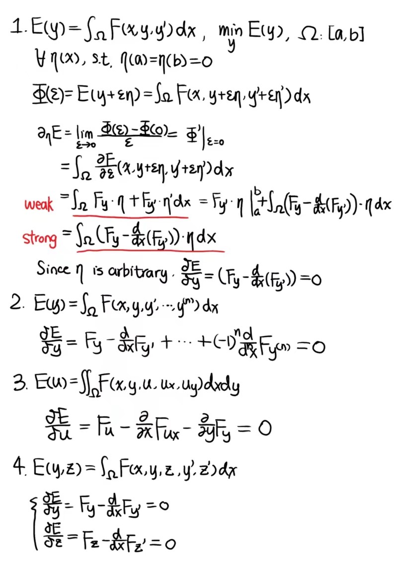
Calculus of variations

Total Variance Denoising

Energy function

minuΩutotal variation +λ2(fu)2dxdy.\min _{u} \iint_{\Omega} \underbrace{\|\nabla u\|}_{\text {total variation }}+\frac{\lambda}{2}(f-u)^{2} d x d y .

E-L equation

δEδu=λ(uf)x(uxux2+uy2)y(uyux2+uy2)=λ(uf)div(uu)\begin{aligned} \frac{\delta E}{\delta u} &=\lambda(u-f)-\frac{\partial}{\partial x}\left(\frac{u_{x}}{\sqrt{u_{x}^{2}+u_{y}^{2}}}\right)-\frac{\partial}{\partial y}\left(\frac{u_{y}}{\sqrt{u_{x}^{2}+u_{y}^{2}}}\right) \\ &=\lambda(u-f)-\operatorname{div}\left(\frac{\nabla u}{\|\nabla u\|}\right) \end{aligned}

Method noise

fTVD{f}=1λcurv(TVD{f})f-T V D\{f\}=-\frac{1}{\lambda} \operatorname{curv}(T V D\{f\})

Solve PDE

Lecture notes (previous course)

Roadmap

Registration

General Formulation

E(ϕ)=d(I,Jϕ)+λL(ϕ)E(\phi) = d(I, J\circ\phi) + \lambda L(\phi)

Similarity metrics

  1. Sum of square distance
d(I,J)=xΩ(I(x)J(x))2d(I, J) = \sum_{x\in\Omega}\left(I(x) - J(x)\right)^2
  1. Cross correlation

    Cross correlation quantifies the linear relationship

cc(I,J)=E[(iμi)(jμj)]E[(iμi)2]12E[(jμj)2]12IμI,JμJσIσJ where {i=I(x),xu(Ωd)j=J(x),xu(Ωd)\begin{aligned} &c c(I, J)=\frac{\mathbb{E}\left[\left(i-\mu_{i}\right)\left(j-\mu_{j}\right)\right]}{\mathbb{E}\left[\left(i-\mu_{i}\right)^{2}\right]^{\frac{1}{2}} \mathbb{E}\left[\left(j-\mu_{j}\right)^{2}\right]^{\frac{1}{2}}} \propto \frac{\left\langle I-\mu_{I}, J-\mu_{J}\right\rangle}{\sigma_{I} \sigma_{J}}\\ &\text { where }\left\{\begin{array}{l} i=I(x), x \sim u\left(\Omega_{d}\right) \\ j=J(x), x \sim u\left(\Omega_{d}\right) \end{array}\right. \end{aligned}
  1. Mutual information
MI(I;J)=KL(P(i,j)P(i)P(j))=ijP(i,j)logP(i,j)P(i)P(j)=ijP(i,j)logP(i,j)iP(i)logP(i)jP(j)logP(j)=H(I,J)+H(I)+H(J)\begin{aligned} \operatorname{MI}(I ; J) &=\mathrm{KL}(P(i, j) \| P(i) P(j)) \\ &=\sum_{i} \sum_{j} P(i, j) \log \frac{P(i, j)}{P(i) P(j)}\\ &=\sum_i\sum_j P(i, j)\log P(i, j) - \sum_i P(i)\log P(i) - \sum_j P(j)\log P(j)\\ &=-H(I, J)+H(I)+H(J) \end{aligned}

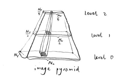
Multi-resolution search

Phase correlation

 Input: I, J I^(u,v)=F(I(x,y))J^(u,v)=F(J(x,y))R(u,v)=I^(u,v)J^(u,v)I^(u,v)J^(u,v)r(x,y)=F1(R(u,v))(τx,τy)=argmax(x,y)Ωr(x,y) Output tx,ty\begin{aligned} &\text { Input: I, J }\\ &\qquad\hat{I}(u, v)=\mathcal{F}(I(x, y)) \\ &\qquad\hat{J}(u, v)=\mathcal{F}(J(x, y)) \\ &\qquad R(u, v)=\frac{\hat{I}(u, v) \hat{J}^{*}(u, v)}{\left|\hat{I}(u, v) \hat{J}^{*}(u, v)\right|} \\ &\qquad r(x, y)=\mathcal{F}^{-1}(R(u, v)) \\ &\qquad \left(\tau_{x}, \tau_{y}\right)=\arg \max _{(x, y) \in \Omega} r(x, y) \\ &\text { Output } t_{x}, t_{y} \end{aligned}

Diffusion model

E(u)=Ω[I(x)J(ϕ(x))]2+λ(u12+u22)dxE(u)=\int_{\Omega}\left[I(x)-J(\phi(x))]^{2}+\lambda\left(\left\|\nabla u_{1}\right\|^{2}+\left\|\nabla u_{2}\right\|^{2}\right) d x\right.

Demon

Optic flow v(x)=(v1(x),v2(x))v(x) = \left(v_1(x), v_2(x)\right)

I(x1,x2,t)=I(x1+v1Δt,x2+v2Δt,t+Δt),(x1,x2)Ω=I(x1,x2,t)+v1ΔtIx1(x1,x2,t)+v2ΔtIx2(x1,x2,t)+ΔtIt(x1,x2,t)+O(Δt2)\begin{align*} I\left(x_{1}, x_{2}, t\right)&=I\left(x_{1}+v_{1} \Delta t, x_{2}+v_{2} \Delta t, t+\Delta t\right), \quad\left(x_{1}, x_{2}\right) \in \Omega\\ &=I\left(x_{1}, x_{2}, t\right)+v_{1} \Delta t \frac{\partial I}{\partial x_{1}}\left(x_{1}, x_{2}, t\right)+v_{2} \Delta t \frac{\partial I}{\partial x_{2}}\left(x_{1}, x_{2}, t\right)+\Delta t \frac{\partial I}{\partial t}\left(x_{1}, x_{2}, t\right)+O\left(\Delta t^{2}\right) \end{align*}

or

vI=Itv\cdot\nabla I = -I_t

Apply to registration

I(x1,x2)=I(x1,x2,0),J(x1,x2)=I(x1,x2,Δt),ϕ(x1,x2)=(x1+v1Δt,x2+v2Δt)(Jϕ)(x1,x2)=J(x1+v1Δt,x2+v2Δt)=I(x1+v1Δt,x2+v2Δt,Δt)=I(x1,x2,0)=I(x1,x2)\begin{align*} I\left(x_{1}, x_{2}\right)&=I\left(x_{1}, x_{2}, 0\right),\\ J\left(x_{1}, x_{2}\right)&=I\left(x_{1}, x_{2}, \Delta t\right),\\ \phi\left(x_{1}, x_{2}\right)&=\left(x_{1}+v_{1} \Delta t, x_{2}+v_{2} \Delta t\right)\\ (J \circ \phi)\left(x_{1}, x_{2}\right)&=J\left(x_{1}+v_{1} \Delta t, x_{2}+v_{2} \Delta t\right)\\&=I\left(x_{1}+v_{1} \Delta t, x_{2}+v_{2} \Delta t, \Delta t\right)\\&=I\left(x_{1}, x_{2}, 0\right)=I\left(x_{1}, x_{2}\right) \end{align*}

And

u(x)=v(x)ΔtuI=IJu(x) = v(x) \cdot \Delta t\\ u\cdot\nabla I=I-J

Solve u(x)=I(x)J(x)I2I(x)u(x)=\frac{I(x)-J(x)}{\|\nabla I\|^{2}} \nabla I(x) or practically

u(x)={0, if I2+(IJ)2<ϵIJ2+(IJ)2I, otherwise u(x)=\left\{\begin{array}{c} 0, \text { if }\|\nabla I\|^{2}+(I-J)^{2}<\epsilon \\ \frac{I-J}{\|\nabla\|^{2}+(I-J)^{2}} \nabla I, \text { otherwise } \end{array}\right.

Update ϕ:ϕϕ(Id+u)\phi: \phi \leftarrow \phi \circ\left(I_{d}+u\right)

LDDMM

Too difficult


Profile picture

Edited by Daniel Shao. Homepage